
Learn the Shape Maker. Surfaces.
- Alexander Alexanov
- May 17, 2020
- 8 min read
To set the shape of the surface, the program uses B-spline surfaces of the third degree. From a mathematical point of view, this means that within one surface area, smoothness is performed along the first derivative (the angle of inclination of the tangent at a point) and continuity along the second derivative (curvature at a point). Surfaces of the third degree are perfectly suited to describe the shape of the vessel. Such surfaces make it possible to achieve the required smoothness and, at the same time, locality of changes.

A feature of these surfaces also lies in the fact that the joining of two surface sections can be performed only with respect to the first derivative (inclination angle). This is quite acceptable in connection between the fore ship surface to a parallel mid body, a flat side or a flat bottom. In the case of joining two curved patches of the surface to each other, the shape of the surface at the junction has an unaesthetic appearance. Very often, such a surface is quite difficult to fix. Therefore, whenever possible, it is recommended to use one curved surface at the fore and aft ship.
Most of the work on changing the shape of the surface is done by changing the position of the points of the control polyhedron. The correct grid location of the control polyhedron is very important to obtain the correct surface smoothing result. Equally important is the uniform distribution of the parameter over the surface grid.
This type of surface is not in vain called sculptural. In general, there are no generally accepted rules for determining the shape of a surface. The hull shape is determined based on the experience and preferences of the designer. The main tool for achieving the desired surface shape in Shape Maker is the control polyhedron. Changing the position of the points of the control polyhedron leads to a regular change in the shape of the surface area. In other words, the Shape Maker does not directly change the shape of the curves, such as frames, waterlines or buttocks, but changes the shape of the surface itself. Surface sections are dynamically displayed on an editable surface section when the position of control points of a polyhedron changes. In this case sections is not an elements in Shape Maker, but just visual representation of surface patch.
Defining surfaces.
Due to the mathematical features of the B-spline surface, the system supports surface patches formed by four, three and two boundary lines.
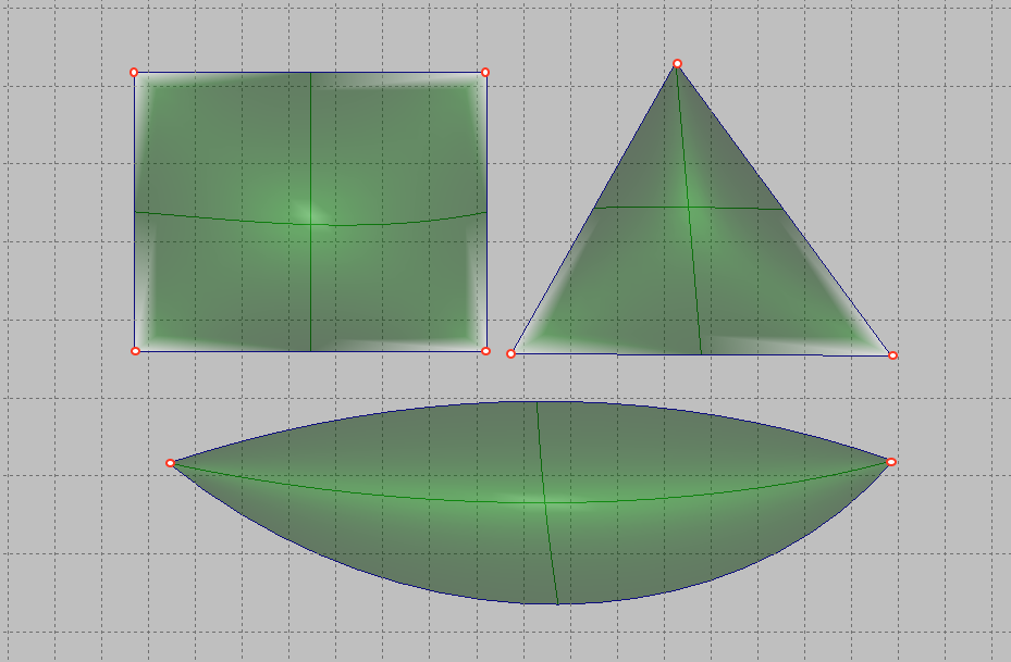
In fact, the case with three and two boundary lines is a special case of a section with four boundary lines, where part of the boundaries degenerate into points. To set the surface, you can use the menu command.

Or a button from the Surface toolbar:

After that, set the lines contour like a sequential line chain and press the Enter button. During the task, marked lines will be highlighted in red. Each subsequent line will be selected as a contour line only if it has a topological connection with the previous one. If required line is not selected it has not topological link to previously selected line. Thi is typical mistake for beginners in Shape Maker. When defining a surface area with three boundary lines, it is important to understand which of the boundaries will be degenerate. There is a simple rule - the first point of the first marked line will be the degenerate boundary of the triangular surface. The sequence of setting the boundaries of the plot is shown in the following figure.

The position of the degenerate surface boundary strongly affects the properties of the triangular surface and the location of the points of the control polyhedron. As shown in the figure below, a part of the line topologically connected to other contour lines through a points on lines can be used as a surface boundary.

Control the number of surface control points.
The number of surface control points in the Shape Maker system is not set by the user, but is generated by the system itself depending on the number of points on the surface boundary curves. Despite the fact that the user can set any number of control points at the borders, it is better to adhere to a certain rule. To understand this, consider how the system calculates how many control points should be inside the surface.
The system uses lines and surfaces of the third degree. This means that the number of intervals of elementary Bezier curves of the third degree inside the B-spline curve is calculated by the formula:
The number of intervals = the number of control points - 3.
In this case, the minimum number of control points of the curve is 4. The extreme points coincide with the beginning and end of the curve. Two other intermediate points define the direction of the tangent and the degree of contact with the tangent at the corresponding end points.
If the curve has four control points, it’s just a Bezier curve with one interval.
If there are five control points, two intervals and so on. The boundary points of the intervals are called the nodes of the curve.
When specifying a surface, the condition of mathematically exact coincidence with the boundary curve is observed. The number of nodes on the surface is calculated as a superposition of nodes of opposite surface boundaries. If the number of nodes at the borders coincides, in this case the surface will have the same number of nodes and, accordingly, the same number of control points.
The resulting surface is shown below build at the top border with five control points and the bottom border with four.

According to the above formula, five control points give us two intervals on the curve connecting in a node. The curve parameter will take the following values:
0.0 - at the starting point of the curve,
1.0 - in the node
2.0 - at the end point of the curve.
The bottom curve has four control points, one interval and no intermediate nodes. When constructing a surface at such boundaries, the Shape Maker automatically creates a node on the lower boundary that corresponds, in terms of the parameter, to a node on the upper boundary. In our case, the value of the node parameter will be - 0.5.
According to the values of the nodes, a surface is built. In our case, in the longitudinal direction on the surface there will be five control points, two surface intervals representing an elementary Bezier surface of the 3rd degree. The line crossing the surface in the vertical direction just represents the line of division into Bezier sections or the line of an equal parameter with a value of 1.0.
Summarizing the above, the surface creation algorithm creates nodes on the curve that correspond to nodes on the opposite curve. A surface is created on curves containing all of these nodes with opposite curves. If the parameters of the nodes on the opposite curves coincide, no new nodes are created and the number of control points on the surface does not increase. In the ideal case, the number of control points on the surface should coincide with the largest number of points on one of the curves. Such conditions create some inconvenience for the user, but have one very important advantage - with this approach to creating surfaces, the common border of two surfaces is mathematically accurate. That is, there are no gaps between the surfaces.
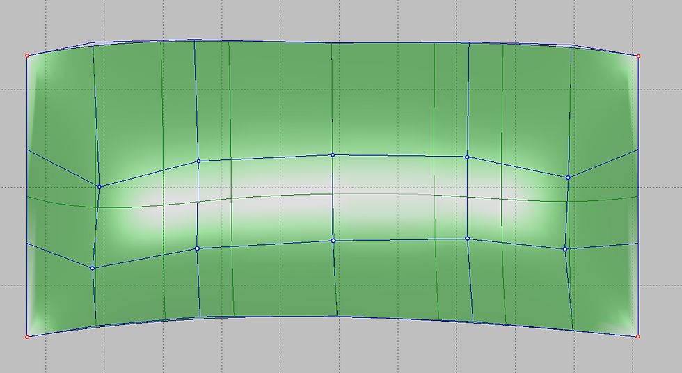
If the number of nodes does not match, then on the surface all nodes corresponding to each of the boundaries are added. This circumstance can dramatically increase the number of control points on the surface and make editing such a surface very difficult. Another very important fact is that mismatched nodes on the surface can be added very close to each other in the parametric space of the surface. The properties of surface control points with an uneven distribution of nodes are very different from uniform distribution and interfere with surface smoothing. This circumstance significantly interferes with surface modeling. The following is an example of a surface where the upper boundary has 6 control points and the lower 5. The resulting surface has 7 control points.
The above problems can be easily avoided if, when defining the boundary lines, combinations of the numbers of control points are used, at which nodes with a uniform distribution of the parameter will be added on the surface. The set of magic numbers of control points is a series: 4 5 7 11 19 35 67 ... According to the formula, the corresponding number of intervals will be 1 2 4 8 16 32 64 .... Accordingly, the nodes on the opposite boundary curves will either coincide or be located along mid-spacing between adjacent nodes. If you use the numbers of this series to set the boundary lines, the resulting surface will always have a uniform distribution of the parameter. In this case, the number of surface points will coincide with the maximum number of points on the boundary curve. This circumstance allows you to set a different number of points on adjacent surfaces. For example, a stem line may have 35 control points. The opposite line of the mid ship bilge radius curve at the entrance to the parallel mid body is only 5 points and the resulting number of points on the bow surface will be 35. In this case, the cylindrical surface of the bilge will have only 5 points. The aft surface mating to the cylindrical part may have, for example, 19 points, if 19 control points are specified on the transom line. It is worth noting that observance of magic numbers is not such a big restriction in the system and is important only for complex curved surfaces. If the surface is flat or cylindrical, then the number of points can be any. If one of the surface boundaries is built on part of the line, it is recommended to bring the point on line strictly to the curve node and calculate the number of control points on the opposite boundary based on the number of nodes on the part of the curve. It will also give a uniform distribution of nodes on the surface. The number of control points on the surface changes when the number of control points on the boundary curves changes. The position of the new control points is selected from the condition of maximum preservation of the surface shape. This allows you to increase the number of points in the process of editing the shape of the surfaces, when the existing number of points is no longer enough.
Surface visualization.
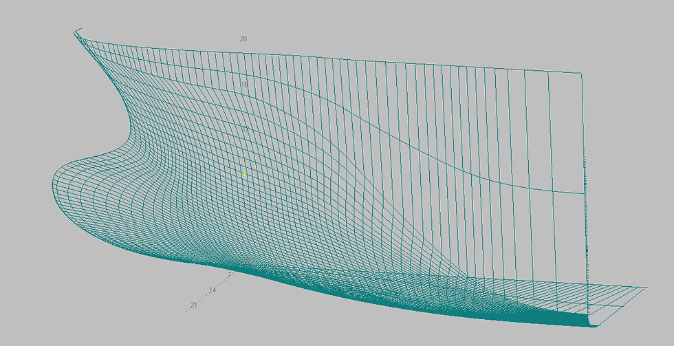
A visual representation of the shape of the surfaces is very important for the smoothing process. The system provides several different options for visualizing surfaces. Lines of equal surface parameter.
These are curves having a constant value of one of the parameters in the parametric representation of the surface. Lines of equal parameter give an idea of how evenly distributed are the points of the control surface polyhedron. The shape of the lines of the equal parameter is automatically recalculated when the points of the control polyhedron change.
Section of the surface by a set of orthogonal planes.
These are curves that are obtained as a result of a surface crossing a set of orthogonal planes. Depending on the current cutting plane, such planes can be frames, waterlines or buttocks. The location of these planes is determined by the grid specified in the model or by the number of sections per depth of the working volume. In the case of visualization of sections along the grid, additional sections are visualized in yellow.

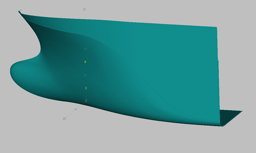
As well as lines of an equal parameter, cross sections are dinamicaly rearranged when the points of the control surface polyhedron change. Shaded surfaces.
One of the options for realistic representation of the surface of the body. For convenience, surface models can also be represented as translucent.
To do this, click on the bar status field with the mouse.


Note that all three of the above visualization options are not independent objects in the system. So, for example, lines of equal parameter or section are not lines that can be edited or deleted. The shape of these lines can only be changed by changing the position of the points of the control surface polyhedron. All three surface options can be turned on simultaneously with the following command.

In the dialog box.

You can also do this by clicking the appropriate button from the Levels: toolbar.


Comments